is an approximation to the root.
A diagram is a good start.
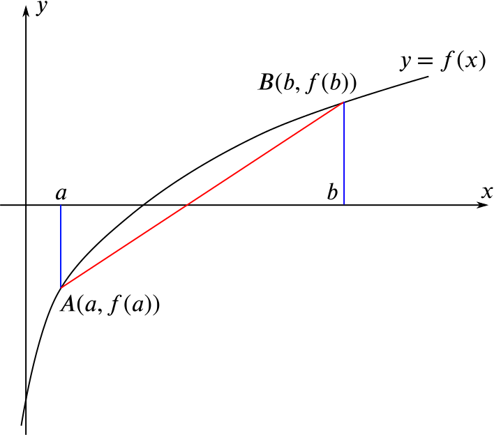
The point where the line \(AB\) meets the \(x\)-axis is usually a better approximation to the root of \(f(x)\) between \(x = a\) and \(x = b\) than either \(x=a\) or \(x=b\).
Approach 1: Find the equation of the line \(AB\)
If a line goes through the points \((p,q)\) and \((r,s)\), its gradient is \(\dfrac{s-q}{r-p}\).
If \((x,y)\) is some point in the plane, then the gradient of the line through \((p,q)\) and \((x,y)\) is \(\frac{y-q}{x-p}\).
Then the point \((x,y)\) will lie on the line if and only if these two gradients are equal, so we can write the equation of the line as \[\frac{y-q}{x-p}=\frac{s-q}{r-p}.\]
Alternatively, we could have used the general formula \(y-y_1=m(x-x_1)\) to write it as \[y-q=\frac{s-q}{r-p}(x-p).\] These are, of course, the same equation.
In our case, therefore, the line between \((a,f(a))\) and \((b,f(b))\) has equation \[\frac{y-f(a)}{x-a}=\frac{f(b)-f(a)}{b-a}.\]
We find the \(x\)-intercept of this line by putting \(y = 0\), giving \[\frac{-f(a)}{x-a}=\frac{f(b)-f(a)}{b-a}.\]
If we now rearrange this to make \(x\) the subject, we first find \[x-a = -f(a)\frac{b-a}{f(b)-f(a)}.\] Adding \(a\) to both sides and putting everything over a common denominator, we find \[x = \frac{af(b) - bf(a)}{f(b) - f(a)},\] as required.
Approach 2: Using similar triangles
If we add a few lines to the above sketch, we find that we have some similar triangles. (This is one of the methods which was explored in In-betweens.)
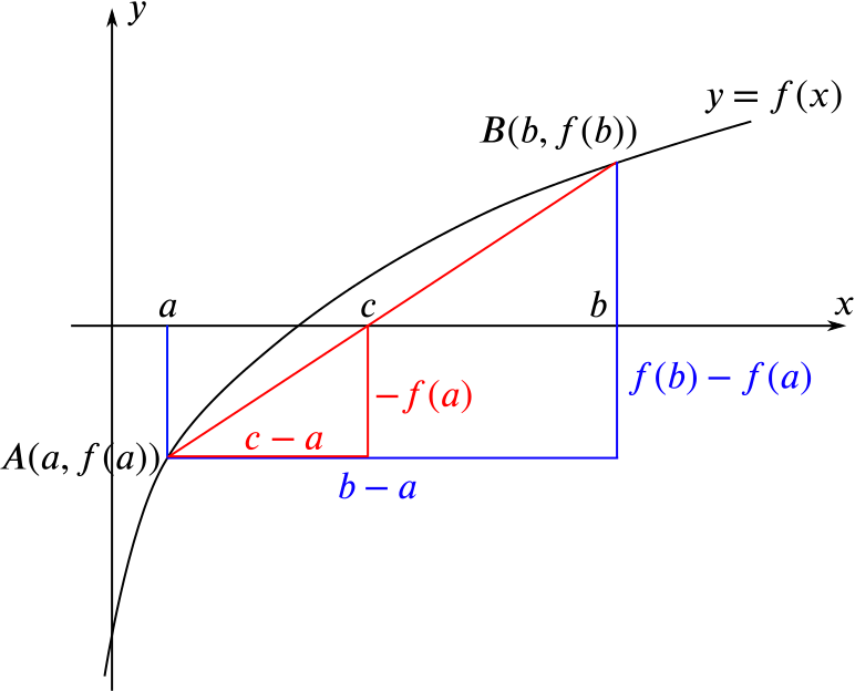
We let \(c\) be the \(x\)-coordinate of the point where \(AB\) crosses the \(x\)-axis, and have indicated various lengths on the diagram. From the similar triangles (the red and blue ones), we find that \[\frac{c-a}{b-a}=\frac{-f(a)}{f(b)-f(a)}.\] Now multiplying both sides by \(b-a\) gives \[c-a=\frac{-(b-a)f(a)}{f(b)-f(a)}.\] Finally, adding \(a\) to both sides and simplifying gives \[c=\frac{af(b)-bf(a)}{f(b)-f(a)}\] as required.
For the equation \(x^2 + x^\frac{1}{2} - 37 = 0\), find two consecutive integers between which a root of the equation lies.
As a first approximation to save us some work, we notice that \(37\approx 6^2\). So trying values of \(x\) near \(6\) seems to be a sensible thing to do.
When \(x=5\), \(x^2 + x^\frac{1}{2} - 37 \approx -9.8\) and when \(x=6\), \(x^2 + x^\frac{1}{2} - 37 \approx 1.4\). So a root lies between \(x=5\) and \(x=6\).
Looking at \(f(x)\), we see that \(f(0) < 0\), and that \(f(x)\) grows without bound as \(x\) increases.
So working upwards from \(x=0\) is guaranteed to lead to a pair of integers \(n\) and \(n+1\) such that \(f(n) < 0\) and \(f(n+1) \ge 0\).
Using the method given in the first part of the question, calculate an approximation to the root, giving three significant figures in your answer.
which, to three significant figures, is \(5.87\). This is an approximation to the root of \(f(x)\) between \(x = a = 5\) and \(x = b = 6\), as required.
It turns out that the true solution is \(5.880060910\!\dotsc\), so our approximation is quite an accurate one in this case.
We can repeatedly apply the above idea.
If we call our first approximation \(x_1\), then we can calculate the value of \(f(x_1)\). It turns out that \(f(x_1)<0\). Since \(f(6)>0\), we can repeat the process with \(x_1\) replacing \(a\) and \(b\) remaining as \(6\).
If we continue doing this, we will progressively home in on the root.
This approach to finding the root of a function is termed the secant method, so named because the line segment \(AB\) is called a secant to the curve, that is, a line segment joining two points on the curve.
It is also known as the linear interpolation method.