Most exercises in mathematics can be seen as construction tasks, in that we are asked to construct a mathematical object that meets certain constraints. Finding a locus is an example, as is solving an equation. To solve the equation \(3x + 7 = 5\) is to construct a number meeting the constraint that multiplying by \(3\) and adding \(7\) results in \(5\). Similarly, the graph of \(y = 3x + 7\) is the set of all coordinates of points \((x, y)\) meeting the constraint that \(y = 3x + 7\).
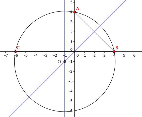
Any statement about (or property of) particular mathematical objects can be regarded as a constraint when we focus on the objects for which the statement is true — the objects that satisfy the constraint. For example, a circle could be described as a closed curve formed by the set of points in a plane that are equidistant from a given point. We can interpret this as a constraint on curves or as a constraint on points in a plane, restricting us to those points that are the same distance from a given point. There are other constraints that define a unique circle and one is featured in Circle of Apollonius…coordinate edition where coordinate geometry is used to explore and solve an ancient geometry problem involving loci. Finding circles also explores which pieces of information are sufficient to determine a single circle.

When we want to understand how something works, we might play with it a bit to see how changing different variables affects behaviour and how behaviour is constrained. In Logarithm lattice, for example, we explore how changing \(a\) or \(b\) affects the value of \(\log_{a}b.\) In How high am I? we explore how an angular change on a Ferris wheel affects the height of a rider and in Sector spirals we consider how changing the radius or angle affects the arc length and area of a circular sector. The basic idea is to learn how a small change in one feature is connected to a change in another feature. When we can quantify these features as variables, we can talk about covariation.
When thinking about graphs of functions, we may ask ‘How does a small increase in the \(x\) variable relate to the change in the \(y\) variable?’ Covariation is at the root of our understanding of gradient, rate of change and optimisation. Relationships between a function and its gradient function can be explored in Gradient match and Can you find…curvy cubics edition.

As noted previously, an equation is an example of a constraint. We can use this to think about what it could mean to solve equations and inequalities. For example, solving \(3x+4=10\) gives \(x=2\), which is a simpler way to express the same constraint. Rewriting an equation offers different ways to see the constraint and is central to Summing to one where Problem 2 asks how many ways we can choose integers \(x\) and \(y\) that satisfy \(\log_{6}x+\log_{6}y=1.\)
As well as equations, we can consider inequalities as constraints. Which is bigger? asks ‘Which is bigger \(\tfrac{2x}{5}\) or \(\tfrac{x}{3}\)?’ and other similar questions. In Two-way algebra we ask students to identify equations or inequalities that satisfy some further property. This is one of several resources based on incomplete two-way tables where we ask students to recognise shared properties among examples and then find further examples. In doing this, students are organising and characterising objects within a larger family, thereby exploring freedom and constraints together.
These examples bring us to the idea of dimension. The \(x,y\)-plane is a \(2\)-dimensional space. Adding an equation such as \(y=x\) or \(x^2+y^2=1\) restricts us to a \(1\)-dimensional space, and imposing another equation restricts us to individual points (or possibly no points). So we see that adding the equational constraints reduces the dimension. If instead we use an inequality such as \(x^2+y^2 <1\) or \(y>x\), we still have a \(2\)-dimensional space, unless the inequality cannot be satisfied.
It can also be interesting to think about the dimension of the space of all objects of a particular kind. For example, if we think of all quadratics of the form \(ax^2+bx+c\) then there are three free parameters or degrees of freedom, and therefore the space of all such quadratics is \(3\)-dimensional. Identifying the number of degrees of freedom is an important idea that lies behind the family of Can you find…? resources, including Can you find… cubic edition and Can you find… trigonometry edition in which we work backwards from constraints to examples or general solutions.

When seeking to construct an object meeting several constraints, it can help to remove one or more constraints. Prime triangles asks which triangular numbers are also prime and how many ways we can justify our answer. Making sense of each constraint separately offers different ways to think about the constraints before combining them.

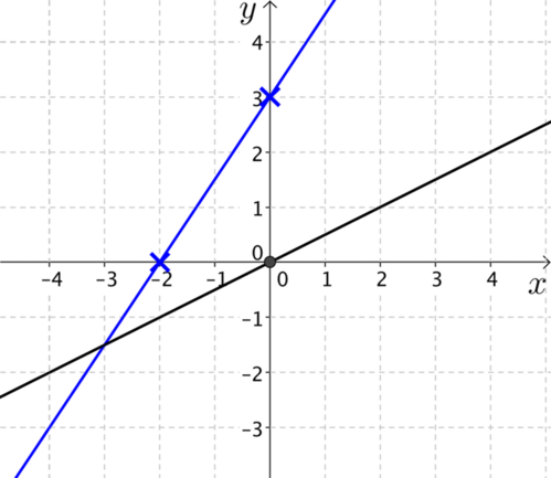
Another example involving multiple constraints is Straight line pairs in which we are asked to construct a pair of straight lines whose \(x\)–intercepts differ by \(2\), whose \(y\)-intercepts differ by \(3\) and whose slopes differ by \(1\). In order to do this, it helps to work with one constraint, then add each constraint on to the class of objects already constructed.

We have described several situations where we are required to construct an object that satisfies one or more constraints. But there are constraints that are not met by any objects — for example, \(x^2 = -1\) is not satisfied by any real number. Often mathematicians explore the possibility of including more objects so that an object meeting a constraint can be constructed. Thus the whole numbers are extended to the integers (by including \(0\) and negatives), to the rationals, to the reals, to the complex numbers and beyond.
Constraints is one of the ideas that we have chosen to highlight in our pervasive ideas.

