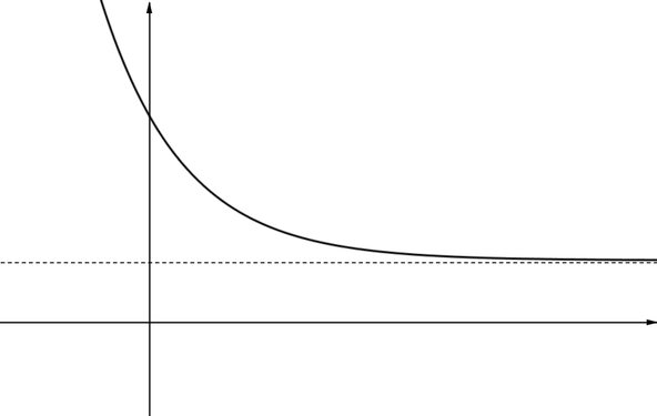
Graph AThis graph has one asymptote which is parallel to the \(x\)-axis. As \(x\) gets larger, the \(y\)-value decreases and the graph gets closer and closer to the asymptote but does not touch it. Part of this graph could model the temperature of a cup of tea as it cools over time. |
|
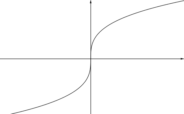
Graph BThis graph does not have an asymptote. The curve gets steeper and closer to the \(y\)-axis as \(x\) gets closer to \(0\), but the \(y\)-axis is a vertical tangent to the curve at \((0,0)\) and is not an asymptote. |
|
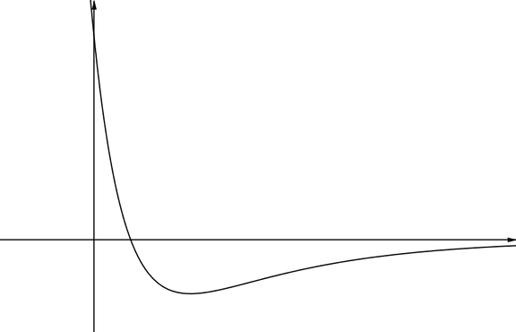
Graph CThe \(x\)-axis is an asymptote of this graph, even though the curve crosses the \(x\)-axis at some point. Part of this graph could model the displacement of a particle on the end of a stretched spring in a highly resistive fluid, such as oil. The particle initially moves quickly until the spring is actually compressed, but then moves slowly back towards the point where the spring is neither stretched nor compressed. This is described as heavy damping. |
|
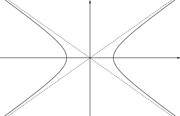
Graph DThis curve has two asymptotes, but neither is parallel to the coordinate axes. They are called ‘oblique’ asymptotes and the two branches of the curve get closer and closer to these as \(x\) gets further away from \(0\). This curve, a hyperbola, is one of the conic sections. These are curves produced by slicing a double cone at different angles. (Note that apart from where the curve crosses the \(x\)-axis, there are always two points on the curve with the same \(x\)-value, so this curve is not the graph of a function.) |
|
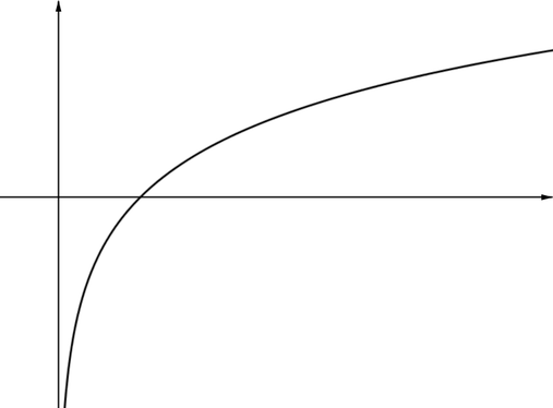
Graph EThe \(y\)-axis is a vertical asymptote and the graph gets closer to this as \(x\) gets closer to \(0\) from the positive side. This function is not defined for \(x=0\) or for negative values of \(x\). It may look as if the graph approaches an oblique asymptote (a line which is not parallel to the axes) as \(x\) gets larger, but this is not the case. Although the value of the function keeps increasing, the graph keeps getting flatter as \(x\) increases. This might suggest that the graph has a horizontal asymptote, but for any horizontal line that you could draw, this graph would actually pass through the line and keep rising as \(x\) increases. |
|
Without more information, such as an equation for the graph, it can be difficult to judge whether a graph has an asymptote. This is one reason we use dotted lines to denote asymptotes on sketch graphs.
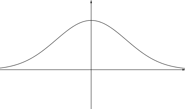
Graph FThe \(x\) axis is a horizontal asymptote for this graph. The function is defined and gives positive values for all values of \(x\), but as \(x\) gets further away from \(0\) the value of the function keeps decreasing and gets closer to \(0\). |
|
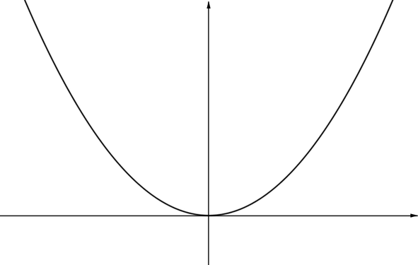
Graph GThis graph does not have any asymptotes, even though the curve gets closer and closer to the \(x\)-axis as \(x\) gets closer to \(0\) from the negative or positive sides. Since the curve meets the \(x\) axis at \((0,0)\) and is horizontal at \((0,0)\), the \(x\)-axis is actually a tangent to the curve, rather than an asymptote. |
|
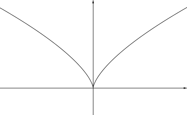
Graph HThis graph doesn’t have any asymptotes. The curve gets steeper and closer to the \(y\)-axis as \(x\) approaches \(0\) from the negative or positive sides, but the curve meets the \(y\)-axis at \((0,0)\) and does not descend further. This is an example of what’s called a ‘cusp’. |
|
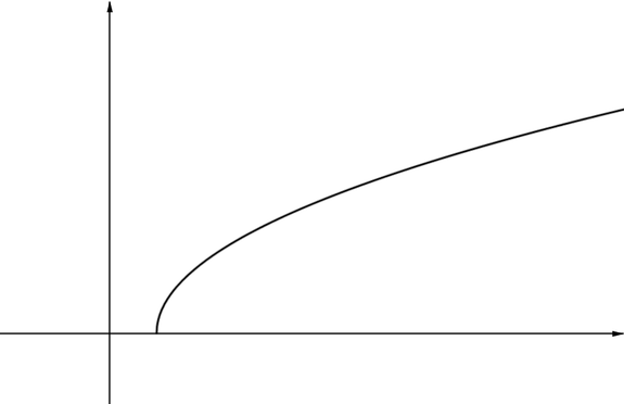
Graph IThis graph doesn’t have any asymptotes. The function is only defined for values of \(x\) greater than a certain value, say for \(x\geq 3\). As \(x\) decreases to \(3\), the curve gets steeper and steeper. The line \(x=3\) is a vertical tangent to the curve at \((3,0)\) rather than an asymptote. |
|
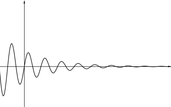
Graph JAlthough this graph crosses the \(x\)-axis multiple times, the \(x\)-axis is an asymptote to the curve. This is because the curve gets arbitrarily close to the \(x\)-axis as \(x\) tends to infinity. That is, if you drew two horizontal lines, one above and one below the \(x\)-axis and as close as you liked to the \(x\)-axis, after some point the curve would be completely contained between these lines and would remain so as \(x\) continued to increase. Part of this graph could model the angle of oscillation of a pendulum over time if we took air resistance into account. |
|
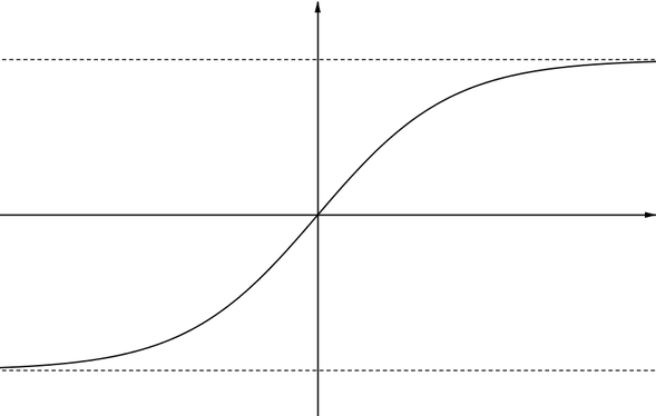
Graph KThis graph has two asymptotes parallel to the \(x\)-axis. As \(x\) tends to infinity the value of the function keeps increasing, but does not go above a certain value. Similarly, as \(x\) tends to negative infinity, the value of the function keeps decreasing, but doesn’t fall below a certain value. |
|
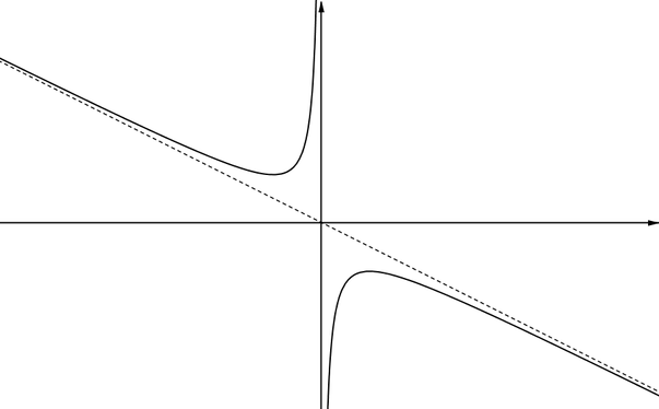
Graph LThis graph has two asymptotes. The \(y\)-axis is an asymptote because as \(x\) approaches \(0\) from the negative side, the function gets larger and larger, tending towards infinity, whereas when \(x\) approaches \(0\) from the positive side the value of the function tends towards negative infinity. There is also an oblique aymptote which the curve gets closer to as \(x\) gets further and further away from \(0\). |
|
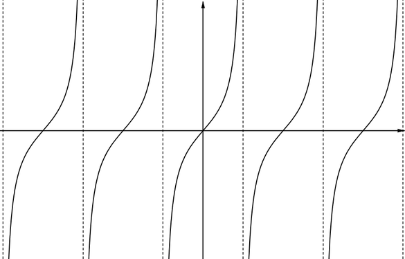
Graph MThis graph has several asymptotes parallel to the \(y\)-axis. For each of these asymptotes, the function approaches infinity on the left side of the asymptote and approaches negative infinity on the right side. |
|
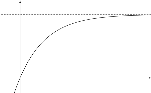
Graph NThis graph has one asymptote parallel to the \(x\)-axis. As \(x\) increases, the value of the function also increases, but it doesn’t go above a certain value. Part of this graph could model the velocity of an object falling from rest if we take air resistance into account. In this situation, the value that \(y\) approaches is often called the terminal velocity. |
|
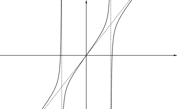
Graph OThis graph has two asymptotes parallel to the \(y\)-axis and on either side of these the value of the function tends to positive or negative infinity. The graph also has an oblique asymptote which the curve approaches as \(x\) gets further away from \(0\). The curve doesn’t cross the vertical asymptotes, but it does cross the oblique asymptote at \((0,0)\). |
|
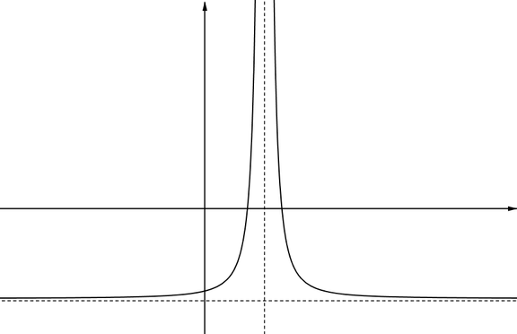
Graph PThe curve approaches the asymptote parallel to the \(x\)-axis as \(x\) tends to positive infinity and as \(x\) tends to negative infinity. There is an asymptote parallel to the \(y\)-axis and on either side of this asymptote the value of the function tends to infinity. |
|

