Below are the discussions of three approaches to finding a more general solution to the problem. They follow the Taking it further section but with more detailed solutions.
This method keeps the calculations simple as it only involves solving linear equations.
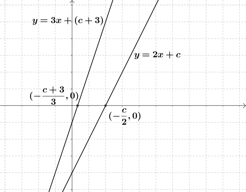
Let’s start by picking a gradient of two and take our first line to be \(y = 2x + c\). Then we can take the case where the second line has a gradient of \(3\) and a \(y\) intercept of \(c + 3\).
When \(y = 0\), the \(x\) values will be \(x= -\dfrac{c}{2}\) and \(x = -\dfrac{c+3}{3}\).
The situation in the graph below is \(-\dfrac{c}{2}-\left(-\dfrac{c+3}{3}\right) = 2\).
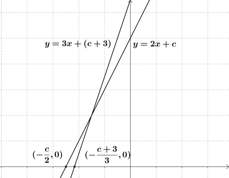
Subtracting the intercepts the other way \(-\dfrac{c+3}{3}--\dfrac{c}{2} = 2\) would come from graphs that look like this.
Solving the equations leads to the solutions of \(c= -6\) and \(c = 18\). So two of the solutions when you start with \(y = 2x + c\) are:
\[y = 2x - 6 \textrm { and } y = 3x - 3,\]
and
\[y = 2x + 18 \textrm { and } y = 3x + 21.\]
We chose the second line to be \(y = (m+1)x + c+3\), which gave us two solutions. Putting the four different options together with the line \(y = 2x+c\) would lead to \(8\) pairs of solutions altogether.
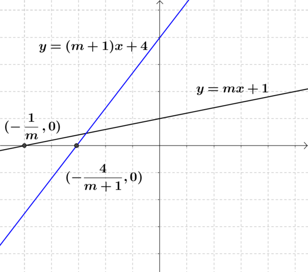
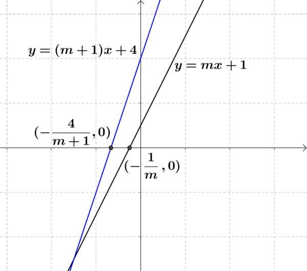
Let us take our first line to be \(y= mx +1\). I will take the second line to be \(y = (m+1)x + 4\). This is only one of four possibilities that the second line could be.
We have our \(y\) intercepts differing by three, we have our gradient differing by one, so we just need the difference of two in our \(x\) intercepts.
When \(y = 0\), \(x = -\dfrac{1}{m}\) in our first line and \(x = -\dfrac{4}{m+1}\) in our second.
Starting with the following equation
\[-\dfrac{4}{m+1}-\left(-\dfrac{1}{m}\right)=2\]
leads to two solutions when you solve the quadratic \(2m^2+5m-1=0\):
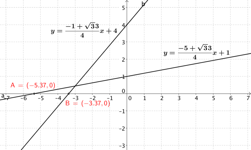
\[m = \dfrac{-5 \pm \sqrt{33}}{4}.\]
So there are two possible values for the gradient, giving us two different pairs of lines. One of these pairs is shown below.
Subtracting the intercepts the other way round leads to the quadratic \(2m^2-m+1=0\) which has no real solutions. This is a nice link to a physical idea of what no solutions means here. Although it is possible to sketch the situation we were trying to solve (see the graph below), it will not be possible to find two lines that fit our constraints.
If you are not convinced, you might like to use the GeoGebra applet to try and find two lines that fit these constraints.
If you change the second line from \(y = (m+1)x + 4\) to \[y = (m+1)x - 2,\] \[y = (m-1)x+4,\] \[y = (m-1)x -2,\]
then you can find the rest of the solutions for this case.
This is not the obvious thing to start with, given our common form for the equation of a straight line which making it easier to think about ‘m’ and ‘c’. However, this actually brings out the relationship between them quite nicely.
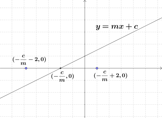
The \(x\) intercept of this line is \(x= -\dfrac{c}{m}\) so the \(x\) intercept of the second line could be \(x=-\dfrac{c}{m}-2\) or \(x = -\dfrac{c}{m}+2\).
This time instead of using \(y = mx+c\) we can use the \(y - y_0=m(x-x_0)\) form as we know the line is travelling through one of the points above.
If we take \((-\dfrac{c}{m}-2, 0)\), then \(y_0=0\), \(x_0=-\dfrac{c}{m}-2\) and we will take the gradient to be \(m+1\). This gives us the equation:
\[y-0 = (m+1)(x - (-\frac{c}{m}-2)),\]
which simplifies to
\[y = (m+1)x + \frac{2m^2+2m+cm+c}{m}.\]
We want our \(y\) intercepts to have a difference of \(3\), so taking our two lines of
\[y = mx+c\]
and
\[y = (m+1)x + \frac{2m^2+2m+cm+c}{m},\]
we can subtract the intercepts to get
\[c - \frac{2m^2+2m+cm+c}{m}=3,\]
which we can rearrange to give us
\[c = -2m^2 - 5m.\]
If you subtracted the equations the other way around then you would get
\[c = m - 2m^2.\]
These are two of the possible expressions for c in terms of m.
There is a lot of scope to investigate this even further.
- You could find all the expressions for c in terms of m, and discuss the symmetry of them. (Graphing them would help).
- You may want to generalise beyond this example, and take the case where the difference between the \(x\) intercepts is \(p\), the \(y\) intercepts is \(q\) and the gradients is \(r\).