Can you find a function that gives the following graph?

There are many ways to approach this problem. We suggest three possibilities below. These are complementary: we could use parts of each of them to reach a conclusion.
- What are the main features of the graph? How can we represent these algebraically?
If we take a step back and look at the graph from a distance, we see that it looks roughly like \(y=x\) when \(x\) is not near zero.
This gives us some hope that we might be able to draw this graph using a function based around polynomials.
Two main features of the graph are the asymptotes (two vertical and one oblique) and the axis crossings, including at the origin. A third key feature is that the function is odd: the graph has rotational symmetry about the origin.
As we have no scale on the graph, we have a certain amount of freedom to choose values for these, as long as they are reasonably consistent with what we see in the graph.
We often need to decide where to focus our attention and how to rework the problem: this is one of the choice points we face when working on a piece of mathematics. Our three approaches each start with the above observations, but take different routes from there.
Approach 1
In this approach, we will focus on the asymptotes.
We will take the asymptotes to be \(x=1\), \(x=-1\) and \(y=x\). (We could have used other numbers, such as \(y=2x\) or \(x=\pm3\), for example.)
Looking at the \(x=1\) asymptote, we see that the graph tends to \(+\infty\) on the left of it and to \(-\infty\) on its right. We can think through our repertoire of graphs related to polynomials: which graphs have a single asymptote with this sort of behaviour?
The graph of \(y=\dfrac{1}{x}\) comes to mind, though we will have to transform it to get it to the right place; something like \(y=\dfrac{1}{x-1}\), or perhaps it is \(y=-\dfrac{1}{x-1}\), should give us the asymptotes we want. We can do something similar near the asymptote \(x=-1\).
These two graphs both tend to \(0\) as \(x\) gets large, though, and we want our graph to tend to \(y=x\) for large \(x\). So maybe we also need to think about the graph of \(y=x\) itself?
Here are the graphs of these three functions:
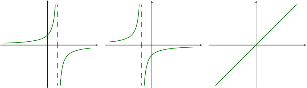
We now have three functions, each of which displays a piece of the behaviour we want from the whole graph. Now all that we need to do is to figure some way of putting these three functions together…
How can you convince yourself that your final answer does have the properties of the graph in the problem?
Approach 2
In this approach, we begin with our initial observation that once \(x\) is large (either positive or negative), the graph looks roughly like \(y=x\). So we can try representing the function as \[\begin{equation} \label{eq:xtimes} y=x\cdot\dfrac{\text{polynomial}}{\text{polynomial}}, \end{equation}\]where the fraction part tends to \(1\) as \(x\) gets large. For this to happen, we need the two polynomials to have the same degree and also the same leading term.
The denominator has to be zero at the vertical asymptotes, which we will take to be \(x=1\) and \(x=-1\), so the polynomial \((x-1)(x+1)=x^2-1\) will do.
This means that the numerator would have to be a quadratic of the form \(x^2+\text{something}\) if this approach works.
Let us now reflect on another question asked in the suggestion:
- Where does the curve cross the axes? How can we represent this information algebraically?
What does this tell us about the quadratic in the numerator?
What will the resulting equation of the graph be? Does this work when you plot it with graph-plotting software?
Approach 3
Similarly to the previous approach, we note that the graph looks like \(y=x\) when \(x\) is large. So we can write the equation of the graph as \[\begin{equation} y=x+\dfrac{\text{polynomial}}{\text{polynomial}}, \end{equation}\]where this time the fraction part tends to zero as \(x\) gets large. For this to happen, the degree of the numerator needs to be less than the degree of the denominator.
To get the asymptotes, we need the denominator to be zero at \(x=\pm1\) as before, so we can again take the denominator to be \(x^2-1\).
We could go two ways from here.
Firstly, we could add the \(x\) and the fraction parts together. This will give us \[y=\dfrac{x(x^2-1)+g(x)}{x^2-1}=\dfrac{x^3-x+g(x)}{x^2-1}\] for some polynomial \(g(x)\) of degree \(0\) or \(1\), so \(y\) will be a cubic divided by \(x^2-1\).
If we can work out the roots of this cubic, we can then write down the whole equation of the graph, and we should be done.
Alternatively, we can think about the fraction part in isolation. Its numerator must be a polynomial of degree \(0\) or \(1\), and the denominator is \(x^2-1\). Also, the whole function is odd, and the initial \(x\) is odd, so the fraction must also be odd.
The denominator is \(x^2-1\), which is an even function; what does this tell us about the numerator?
Does this give us enough information to find an equation for the graph?
How do these approaches illuminate different aspects of the graph?
Which aspects are most easily generalised?