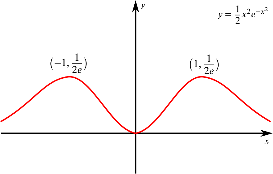
The curve \(C_1\) passes through the origin in the \(x\text{-}y\) plane and its gradient is given by \[ \frac{dy}{dx}=x(1-x^2)e^{-x^2}.\] Show that \(C_1\) has a minimum point at the origin and a maximum point at \((1,\frac{1}{2}e^{-1})\). Find the coordinates of the other stationary point. Give a rough sketch of \(C_1\).
\[\frac{dy}{dx}=x(1-x^2)e^{-x^2}.\] This is zero when \(x=0,\pm 1\). To classify these stationary points we need the second derivative:
\[\begin{align*}
\frac{d^2y}{dx^2} &= (1-x^2)e^{-x^2}+x(-2x)e^{-x^2}-2x^2(1-x^2)e^{-x^2}\\
&= (1-5x^2+2x^4)e^{-x^2}.
\end{align*}\]
Thus
\[\begin{align*}
y''(0) &= 1 > 0 \quad \Longrightarrow \quad \text{this is a minimum point,} \\
y''(-1)=y''(1) &= (1-5+2)e^{-1} = -\frac{2}{e} < 0 \quad \Longrightarrow \quad \text{these are maximum points.}
\end{align*}\]
Since we know the curve passes through the origin, \((0,0)\) must be a minimum point.
To find the coordinates of the other stationary points we need to know the values of \(y(\pm1)\) which requires us to integrate the given expression. There are (at least) two different ways of doing this.
Let’s try to integrate \(x(1-x^2)e^{-x^2}\) by parts.
Remember that the formula for integration by parts is \[
\int u\frac{dv}{dx}\:dx=uv-\int v\frac{du}{dx}\:dx
\]
Notice that \(xe^{-x^2}\) is the derivative of \(-\frac{1}{2}e^{-x^2}\). So let’s set \[
\frac{dv}{dx}=xe^{-x^2}, \implies v=-\frac{1}{2}e^{-x^2},
\] and \[
u=1-x^2, \implies \frac{du}{dx}=-2x.
\]
So we have that
\[\begin{align*}
y=\int x(1-x^2)e^{-x^2}\:dx &= -\frac{1}{2}(1-x^2)e^{-x^2}-\int x e^{-x^2}\:dx\\
&=-\frac{1}{2}(1-x^2)e^{-x^2}+\frac{1}{2}e^{-x^2}=\frac{1}{2}x^2e^{-x^2}.
\end{align*}\]
Notice that we don’t need to add a constant because the curve passes though the origin (or we could say the constant of integration is 0).
We’ll guess at a solution of the form \(y=(ax^2+bx+c)e^{-x^2}\).
From the work above finding \(\frac{d^2y}{dx^2}\) we can see that differentiating an expression of this form tends to increase the degree of the leading polynomial by one. So when integrating, we expect the leading cubic to become a quadratic.
Thus \[y=\frac{1}{2}x^2e^{-x^2},\] which we can see satisfies the boundary condition \(x=0,\,y=0.\)
Our maxima are therefore found at \(\left(\pm 1,\dfrac{1}{2e}\right)\). Furthermore, the function is even, that is \(f(-x)=f(x)\) for all \(x\); and as \(x \rightarrow \pm\infty\), \(y \rightarrow 0\).
The curve \(C_2\) passes through the origin in the \(x\text{-}y\) plane and its gradient is given by \[ \frac{dy}{dx}=x(1-x^2)e^{-x^3}.\] Show that \(C_2\) has a minimum point at the origin and a maximum point at \((1,k)\), where \(k>\frac{1}{2}e^{-1}\).
So now \[\frac{dy}{dx}=x(1-x^2)e^{-x^3}.\]
Note the change from \(-x^2\) to \(-x^3\) in the power of \(e\) means this becomes a really hard differential equation to solve.
The methods we used above both fail. Fortunately we can complete the question without directly solving this equation.
The stationary points are again at \(x=0,\,\pm 1\). Classifying these:
\[\begin{align*}
\frac{d^2y}{dx^2} &= \left(1-x^2\right)e^{-x^3} -2x^2e^{-x^3} -3x^3\left(1-x^2\right)e^{-x^3} \\
&= \left(1-3x^2-3x^3+3x^5\right)e^{-x^3}.
\end{align*}\]
Thus
\[\begin{align*}
y''(0) &= 1 > 0 \quad \Longrightarrow \quad \text{this is a minimum point,} \\
y''(\pm1) &= (1-3\mp3\pm3)e^{-1} = -\frac{2}{e} < 0 \quad \Longrightarrow \quad \text{these are maximum points.}
\end{align*}\]
Now we need to show the maximum point at \((1,k)\) satisfies \(k>\frac{1}{2}e^{-1}\). We cannot evaluate the function directly, but we know that the curve passes through the origin, like \(C_1\), and that \(C_1\) has a maximum at \((1,\frac{1}{2}e^{-1})\). So we know \(C_1\) reaches this point, and we want to show \(C_2\) goes above it. For \(0<x<1\), we have:
So the derivative of \(C_2\) is greater than that of \(C_1\) in this range. That means that \(C_2\)’s \(y\) value is “growing” faster than \(C_1\)’s between the origin and the maximum point at \(x=1\), so its maximum point will have greater \(y\)-coordinate, that is to say, the maximum occurs at \((1,k)\), where