How can we find the formula for the great circle distance?
In Lost but lovely: the haversine we explored great circle distances on the Earth and looked at the haversine formula for calculating them: \[\mathop{\mathrm{haversin}} \left(\frac{d}{R}\right) = \mathop{\mathrm{haversin}} (\phi_2-\phi_1) + \cos{\phi_1}\cos{\phi_2} \mathop{\mathrm{haversin}} (\lambda_2-\lambda_1).\]
Recall that in this formula, we are finding the great circle distance \(d\) between two points \(P\) and \(Q\) which have latitudes \(\phi_1\) and \(\phi_2\) and longitudes \(\lambda_1\) and \(\lambda_2\) respectively. The radius of the Earth (or sphere) is \(R\), and the haversine is defined by \[\mathop{\mathrm{haversin}} x=\sin^2\left(\frac{x}{2}\right).\] (On the left hand side of the first equation, \(\frac{d}{R}\) is thought of as an angle in radians.)
So we can rewrite the haversine formula in more familiar notation as \[\sin^2{\left(\frac{d}{2R}\right)} = \sin^2{\left(\frac{\phi_2-\phi_1}{2}\right)} + \cos{\phi_1}\cos{\phi_2} \sin^2{\left(\frac{\lambda_2-\lambda_1}{2}\right)}.\]
In this piece, we explore where this formula comes from, and why navigators might have used the unfamiliar haversine rather than ordinary sines and cosines in their calculations.
Preliminaries
We can use any units of distance that we wish when we do our calculations: changing units does not affect the value of \(\frac{d}{R}\) (as long as we use the same units for both \(d\) and \(R\)). Most conveniently, we can choose units so that the radius of the earth is \(R=1\), meaning that we are working with a unit sphere. Then the haversine formula becomes
\[\begin{equation}
\label{eq:haversine}
\mathop{\mathrm{haversin}} d = \mathop{\mathrm{haversin}} (\phi_2-\phi_1) + \cos{\phi_1}\cos{\phi_2} \mathop{\mathrm{haversin}} (\lambda_2-\lambda_1)
\end{equation}\]
or
\[\begin{equation}
\label{eq:haversinesine}
\sin^2{\left(\frac{d}{2}\right)} = \sin^2{\left(\frac{\phi_2-\phi_1}{2}\right)} + \cos{\phi_1}\cos{\phi_2} \sin^2{\left(\frac{\lambda_2-\lambda_1}{2}\right)},
\end{equation}\]
which looks a little simpler. We will work with these forms throughout.
The great circle distance, \(d\), is the shorter arc joining two points on a great circle. We can also consider the chord (straight line) joining the two points, and we let its length be \(C\).
We can immediately observe some relationships between \(d\), \(C\) and the angle \(\sigma\) (measured in radians) that the great circle arc makes with the centre of the sphere: we have \(d=\sigma\) (as the radius is \(1\)), and by drawing the isosceles triangle \(POQ\), we see that \(C=2\sin\bigr(\frac{\sigma}{2}\bigr)\):
Putting these together by eliminating \(\sigma\), \[\frac{C}{2}=\sin\left(\frac{d}{2}\right).\] If we square this and multiply by \(4\), we get an alternative expression:
\[\begin{equation}
\label{eq:chordhaversine}
C^2=4\sin^2\left(\frac{d}{2}\right)=4\mathop{\mathrm{haversin}} d.
\end{equation}\]
We now offer four approaches to deducing the haversine formula. The first two of these use coordinates, so we begin with this.
Coordinates
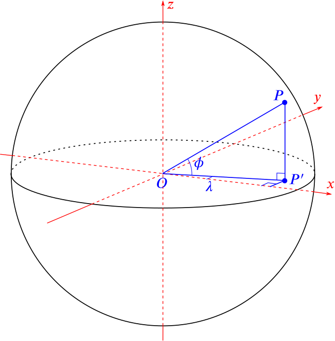
Given a point on the unit sphere with latitude \(\phi\) and longitude \(\lambda\), we can calculate the corresponding Cartesian coordinates, as shown in the following diagram.
What are the Cartesian coordinates of \(P\) (that is, its \((x,y,z)\) coordinates)?
From the diagram we can see that
\[\begin{align*}
&\text{firstly}& z &= \sin \phi\\
&\text{and}& OP' &= \cos \phi,\\
&\text{so}& x &= \cos \phi \cos \lambda\\
&\text{and}& y &= \cos \phi \sin \lambda.
\end{align*}\]
Once we know the Cartesian coordinates of the points \(P\) and \(Q\) with latitudes \(\phi_1\) and \(\phi_2\) and longitudes \(\lambda_1\) and \(\lambda_2\) respectively, we can calculate the differences in the \(x\), \(y\) and \(z\) coordinates of the two points and use those to calculate appropriate distances or angles in order to find \(d\).
However, the expressions are going to become quite cumbersome with so many variables, so we look for a way to simplify things before going further.
One trick is to notice that the distances and angle \(\sigma\) all remain unchanged if we rotate the sphere about the north-south axis. This only changes the longitudes of the points, so we could rotate it until \(P\) has longitude \(0\) and \(Q\) has longitude \(\lambda_2-\lambda_1\), which we will call \(\Delta\lambda\) (the difference between the \(\lambda\)s).
Then the coordinates of \(P\) and \(Q\) become:
\[\begin{align*}
P &= (\cos\phi_1, 0, \sin\phi_1)\\
Q &= (\cos\phi_2\cos(\Delta\lambda), \cos\phi_2\sin(\Delta\lambda), \sin\phi_2).
\end{align*}\]
We could perhaps try rotating further so that \(P\) lies at the north pole, say, but it is not clear what would happen to \(Q\) if we did that, so we will stop rotating at this point.
Approach 1: Pythagoras and trigonometry
What is the distance between \(P\) and \(Q\)?
Using Pythagoras’s theorem, the square of the distance is given by
\[\begin{align*}
(\cos\phi_2\cos(\Delta\lambda)-\cos\phi_1)^2&+(\cos\phi_2\sin(\Delta\lambda))^2+(\sin\phi_2-\sin\phi_1)^2\\
&=\cos^2\phi_2\cos^2(\Delta\lambda)-2\cos\phi_1\cos\phi_2\cos(\Delta\lambda)+\cos^2\phi_1+\cos^2\phi_2\sin^2(\Delta\lambda)\\
&\quad +\sin^2\phi_2-2\sin\phi_1\sin\phi_2+\sin^2\phi_1\\
&=\cos^2\phi_2 - 2\cos\phi_1\cos\phi_2\cos(\Delta\lambda) -2\sin\phi_1\sin\phi_2 +1+\sin^2\phi_2\\
&=2 - 2\cos\phi_1\cos\phi_2\cos(\Delta\lambda) -2\sin\phi_1\sin\phi_2.
\end{align*}\]
(We have used the identity \(\sin^2x+\cos^2x=1\) a few times here.)
Since the distance between them is actually \(C\), we have \[C^2=2 - 2\cos\phi_1\cos\phi_2\cos(\Delta\lambda) -2\sin\phi_1\sin\phi_2.\]
We can take the square root of this to find \(C\) if we wish to.
Recalling from above that \(\frac{C}{2}=\sin\bigl(\frac{d}{2}\bigr)\), can you use this to obtain an expression for \(\sin^2\bigl(\frac{d}{2}\bigr)\) as it appears in the haversine formula (equation \(\eqref{eq:haversinesine}\) above)?
We have to divide our previous expression by \(4=2^2\) to get \[\sin^2\bigl(\tfrac{d}{2}\bigr)=\bigl(\tfrac{C}{2}\bigr)^2=\tfrac{1}{2}\bigl(1 - \cos\phi_1\cos\phi_2\cos(\Delta\lambda) -\sin\phi_1\sin\phi_2\bigr).\]
Comparing this with the expression we want, we are reminded of the half-angle formula \(\sin^2\frac{x}{2}=\frac{1}{2}(1-\cos x)\) and also the compound angle formula \[\cos(\phi_2-\phi_1)=\cos\phi_2\cos\phi_1+\sin\phi_2\sin\phi_1.\]
Since we know the coordinates of \(P\) and \(Q\), we also know the vectors \(\mathbf{p}=\overrightarrow{OP}\) and \(\mathbf{q}=\overrightarrow{OQ}\). They each have unit length, so the angle between them, \(\sigma\), is given by \(\cos\sigma=\mathbf{p}\cdot\mathbf{q}\).
Can you use this to find an expression for \(\sin^2\bigl(\frac{d}{2}\bigr)\)?
Recalling that \(P=(\cos\phi_1, 0, \sin\phi_1)\) and \(Q=(\cos\phi_2\cos(\Delta\lambda), \cos\phi_2\sin(\Delta\lambda), \sin\phi_2)\), we have
\[\begin{align*}
\cos\sigma&=\mathbf{p}\cdot\mathbf{q}\\
&=\cos\phi_1\cos\phi_2\cos(\Delta\lambda)+0+\sin\phi_1\sin\phi_2.
\end{align*}\]
Now \(\sigma=d\), so we can use the formula \(\sin^2\frac{x}{2}=\frac{1}{2}(1-\cos x)\) to write down \[\sin^2\bigl(\tfrac{d}{2}\bigr)=\tfrac{1}{2}\bigl(1-\cos\phi_1\cos\phi_2\cos(\Delta\lambda)-\sin\phi_1\sin\phi_2\bigr).\]
We can then continue exactly as in Approach 1.
Approach 3: Spherical trigonometry
Just as there are sine and cosine rules for triangles in the plane, there are similar rules for triangles on a sphere.
Here is a drawing of a spherical triangle:
The angles \(A\), \(B\) and \(C\) are the angles at the vertices \(A\), \(B\) and \(C\) of the triangle, while \(a\), \(b\) and \(c\) are the side lengths as usual. But if we take the sphere to have radius \(1\), then they can also be thought of as angles: \(a\) is the angle \(\angle BOC\), for example. We therefore assume the sphere to have radius \(1\) from now on.
There are two spherical cosine rules and one spherical sine rule, which are:
spherical cosine rule (1): \[\cos a=\cos b\cos c+\sin b\sin c\cos A\] (and similar equations with \(a\), \(b\), \(c\) and \(A\), \(B\), \(C\) permuted)
spherical cosine rule (2): \[\cos A=-\cos B\cos C+\sin B\sin C\cos a\] (and similar equations with \(a\), \(b\), \(c\) and \(A\), \(B\), \(C\) permuted)
spherical sine rule: \[\dfrac{\sin A}{\sin a}=\dfrac{\sin B}{\sin b}=\dfrac{\sin C}{\sin c}\]
Can you use this information to find an expression for \(\cos\sigma\) and then \(\sin^2\bigl(\frac{d}{2}\bigr)\) in our case?
If we take \(A\) to be the north pole, \(B\) to be our point \(P\) and \(C\) to be our point \(Q\), then \(a=\sigma\), \(b=\frac{\pi}{2}-\phi_2\) (sometimes called the colatitude of \(Q\) – can you see why?), \(c=\frac{\pi}{2}-\phi_1\) and \(A=\Delta\lambda\).
This gives another way of seeing why only the difference between the longitudes is important.
So we know \(b\), \(c\) and \(A\), and we want to find \(a\), meaning that we can use the first spherical cosine rule. This immediately gives
\[\begin{align*}
\cos\sigma&=\cos(\tfrac{\pi}{2}-\phi_2)\cos(\tfrac{\pi}{2}-\phi_1)+\sin(\tfrac{\pi}{2}-\phi_2)\sin(\tfrac{\pi}{2}-\phi_2)\cos(\Delta\lambda)\\
&=\sin\phi_1\sin\phi_2+\cos\phi_1\cos\phi_2\cos(\Delta\lambda).
\end{align*}\]
As in Approach 2, we have \(\sigma=d\), so we can use the formula \(\sin^2\frac{x}{2}=\frac{1}{2}(1-\cos x)\) to write down \[\sin^2\bigl(\tfrac{d}{2}\bigr)=\tfrac{1}{2}\bigl(1-\cos\phi_1\cos\phi_2\cos(\Delta\lambda)-\sin\phi_1\sin\phi_2\bigr).\]
Again, we can then continue exactly as in Approach 1.
Approach 4: Using haversines directly
The above approaches have all proven the haversine formula via the familiar sine and cosine functions. In this approach, we will use equation \(\eqref{eq:chordhaversine}\) above for the length of a chord in terms of the haversine function: \[C^2=4\mathop{\mathrm{haversin}} d,\] where \(d\) is the great circle distance (or angle subtended) and \(C\) is the corresponding chord length.
We wish to find the great-circle distance \(d\) between the points \(P\) and \(Q\) with latitudes \(\phi_1\) and \(\phi_2\) and longitudes \(\lambda_1\) and \(\lambda_2\) respectively.
By thinking about symmetry, we are prompted to also consider the points \(R\) and \(S\) with latitudes \(\phi_1\) and \(\phi_2\) but with swapped longitudes \(\lambda_2\) and \(\lambda_1\) respectively. This gives us the following configuration:
In this diagram, the blue lines are all straight chords (though an optical illusion makes it look otherwise), and the red line is the great circle between \(P\) and \(Q\).
Can you use this diagram to deduce the haversine formula?
The first thing to observe is that the lines \(PR\) and \(SQ\) are parallel. This is because the circles at latitudes \(\phi_1\) and \(\phi_2\) are just scaled versions of each other. This means that the quadrilateral \(PRQS\) is actually planar and a trapezium. Furthermore, the lengths \(PS\) and \(RQ\) are the same by construction. The trapezium is therefore an isosceles trapezium. We can redraw it like this:
We can work out the length \(e\) directly, as the great circle between \(P\) and \(S\) is the line of longitude, so \[e^2=4\mathop{\mathrm{haversin}}(\phi_2-\phi_1).\] (It might be that the angle between \(P\) and \(S\) is actually \(\phi_1-\phi_2\), but as \(\mathop{\mathrm{haversin}}(-x)=\mathop{\mathrm{haversin}}x\), it makes no difference.)
If \(P\) and \(R\) were on the equator, we would have \(PR^2=4\mathop{\mathrm{haversin}}(\lambda_2-\lambda_1)\) in the same way. But the circle of latitude \(\phi_1\) has radius \(\cos\phi_1\), so scaling by a factor of \(\cos\phi_1\) gives us
\[\begin{align*}
b&=2\cos\phi_1\sqrt{\mathop{\mathrm{haversin}}(\lambda_2-\lambda_1)}\\
a&=2\cos\phi_2\sqrt{\mathop{\mathrm{haversin}}(\lambda_2-\lambda_1)},
\end{align*}\]
with the second line following similarly.
We can finish the argument off with two applications of Pythagoras’ theorem on the triangles \(PQT\) and \(QTR\):
\[\begin{align*}
C^2 &= h^2 + \left(\frac{b+a}{2}\right)^2\\
e^2 &= h^2 + \left(\frac{b-a}{2}\right)^2
\end{align*}\]
Eliminating \(h^2\) from these gives \[C^2 = e^2 + \left(\frac{b+a}{2}\right)^2 - \left(\frac{b-a}{2}\right)^2 = e^2 + ab.\] But \(C^2=4\mathop{\mathrm{haversin}} d\) and we have now worked out \(e^2\), \(a\) and \(b\), so substituting for these gives \[4\mathop{\mathrm{haversin}} d = 4\mathop{\mathrm{haversin}} (\phi_2-\phi_1) + 4\cos\phi_1\cos\phi_2\mathop{\mathrm{haversin}} (\lambda_2-\lambda_1).\] Dividing by \(4\) then gives the haversine formula.
How do these four approaches compare?
Why use haversines?
Surely we could just use \(\cos\bigl(\frac{d}{R}\bigr)=\cos\phi_1\cos\phi_2\cos(\Delta\lambda)+\sin\phi_1\sin\phi_2\) to calculate great circle distances, as we found in Approaches 2 and 3? Why would anyone need the haversine? (We have reinserted the radius \(R\) here, as practical calculations will use standard units of measurement. Also, a reason is given in Lost but lovely: the haversine for introducing the haversine, but that was just to simplify the formula involving three occurrences of \(\sin^2\frac{x}{2}\).)
Navigators in the past would have had to make do with tables and slide rules: there were no calculators. So what would happen if we try to work out the distance between Dover and Calais, say, using the two different formulae, but restricting ourselves to the limited calculating tools of the past?
Here is some relevant information:
Dover: latitude \(\quantity{51.15^\circ}{N}\), longitude \(\quantity{1.33^\circ}{E}\)
Calais: latitude \(\quantity{50.97^\circ}{N}\), longitude \(\quantity{1.85^\circ}{E}\)
Radius of the Earth: \(\quantity{6378}{km}\)
And trigonometric values, accurate to 4 significant figures or 4 decimal places:
Using these values, calculate the great circle distance from Calais to Dover using the two different formulae (and you can use a calculator for the multiplications, and for working out the final inverse cosine and haversine). To truly emulate the past, round all of your intermediate calculations to 4 significant figures as well.
Using the formula \[\cos\left(\frac{d}{R}\right)=\cos\phi_1\cos\phi_2\cos(\Delta\lambda)+\sin\phi_1\sin\phi_2\] we can calculate as follows (working to 4 significant figures):
This is quite unfortunate: we have lost too much information because \(\cos(\Delta\lambda)\) is so close to \(1\). In fact, it is \(0.9999588\) to 7 decimal places, but even that increased accuracy would be of no help if we continue to work to 4 decimal places further on. Tables were not available with that level of accuracy, so this formula is useless for calculating short distances.
On the other hand, the haversine formula is \[\mathop{\mathrm{haversin}} \left(\frac{d}{R}\right) = \mathop{\mathrm{haversin}} (\phi_2-\phi_1) + \cos{\phi_1}\cos{\phi_2} \mathop{\mathrm{haversin}} (\lambda_2-\lambda_1).\] So we can calculate \(d\) (remembering at the end that we need to work in radians when taking the inverse haversine):
And this agrees to 4 significant figures with the value calculated on a calculator, because we have not lost any significant accuracy when working with the haversine of small angles.
The actual great circle distance between Dover and Calais is this, plus or minus a couple of kilometers, as the latitude and longitude are only accurate to \(0.01^\circ\); they would need to be more precise to give a more accurate answer.
The reason the simple formula fails for small distances is that if \(\Delta\lambda\) is small, then \(\cos(\Delta\lambda)\) is almost exactly \(1\). Then the formula becomes \[\cos\left(\frac{d}{R}\right)\approx\cos\phi_1\cos\phi_2+\sin\phi_1\sin\phi_2=\cos(\phi_2-\phi_1).\] If the difference in latitudes, \(\phi_2-\phi_1\), is also small, then this gives \(\cos\bigl(\frac{d}{R}\bigr)\approx1\), and so \(\frac{d}{R}\approx0\).
What the haversine formula does instead is to work in terms of the sines of the differences between the latitudes and longitudes. If \(\Delta\lambda\) is small, then \(\sin(\Delta\lambda)\approx\Delta\lambda\) (as long as we are working in radians), so working to 4 significant figures will still be very accurate.