What’s the shortest route between two points? What if the two points are, say, London and San Francisco, and you’d like to travel from one to the other? The straight line that connects them in three-dimensional space passes through the Earth, so to travel along it you would have to dig a tunnel. In practice you have to travel across the surface of the Earth (or at least near the surface of the Earth if you are in a plane). So the question now is: what is the shortest route between two points on the surface of a sphere?
Here is the answer: the shortest route between two points on a sphere is along an arc of a great circle. A great circle is a circle drawn on the surface of the sphere, centred on the same point as the sphere and having the same radius. An example is the equator of the Earth. Out of all the circles you could draw on the sphere a great circle has the largest radius, spanning right around the fattest part of the sphere. The intersection of a plane which contains the centre of the sphere and the sphere is a great circle.
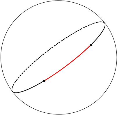
Show that there is exactly one great circle passing through any two points \(P\) and \(Q\) on the sphere that are not antipodal (that don’t lie exactly opposite each other, as the North and South pole do).
Two points \(P\) and \(Q\) divide the great circle they lie on into two arcs. The shorter of these arcs gives the shortest path between the two points.
So how do you calculate the great circle distance, as it is called, between two points \(P\) and \(Q\) on the Earth? First, recall that the locations of the two points are given by their latitudes (see here for how to calculate latitudes) \(\phi_1\) and \(\phi_2\) and their longitudes (and here for how to calculate longitudes) \(\lambda_1\) and \(\lambda_2\). Let’s write \(R\) for the radius of the Earth, which is roughly \(\quantity{6378}{km}\). The great circle distance \(d\) between \(P\) and \(Q\) comes from the formula
\[\begin{equation} \label{eq:1} \sin^2{\left(\frac{d}{2R}\right)} = \sin^2{\left(\frac{\phi_2-\phi_1}{2}\right)} + \cos{\phi_1}\cos{\phi_2} \sin^2{\left(\frac{\lambda_2-\lambda_1}{2}\right)} \end{equation}\](where \(\frac{d}{2R}\) is treated as an angle measured in radians). Several derivations of this formula can be found in The great circle distance.
Rearrange equation \(\eqref{eq:1}\) to make the great circle distance \(d\) the subject of the formula.
You will agree that this isn’t the neatest of formulae. Imagine being a sailor hundreds of years ago, who had to work out the great circle distance between places, but didn’t have a calculator! In those days people used tables which told them the values of the trigonometric functions: given a value of \(x\), those tables told you the values of \(\cos x\) and \(\sin x\), and vice versa. Working out the great circle distance using the formula above would have involved a lot of looking up, as well as adding, multiplying, dividing, squaring and taking a square root.
But luckily there was help at hand. People invented a new trigonometric function, called the haversine (the term comes from “half versed sine”), which is defined as
\[\mathop{\mathrm{haversin}}\nolimits (x) = \sin^2{\left(\frac{x}{2}\right)}.\]
It makes the expression above look a little simpler and sailors used this, along with tables of the haversine function, instead of the sine function, to work out the great circle distance. This saved them having to work out \(\sin^2 x\) many times.
Write equation \(\eqref{eq:1}\) above replacing components by the haversine function where possible.
The function \(\sin^2\left(\frac{x}{2}\right)\) comes up quite frequently in mathematics. It turns out that \[2\sin^2\left(\frac{x}{2}\right) = 1 - \cos{x}.\] There is more relating to this double angle formula at Trigonometry: Compound Angles.
This illustrates the connection to the versine, which came up in Have a sine.
Writing \(\mathop{\mathrm{haversin}}\nolimits ^{-1}\) for the inverse of the haversine function, make \(d\) the subject of your equation involving haversine.
Now that we have an equation to work out the great circle distance, we can try using the tables of values just like sailors of old. Helpfully, the tables can be used not only to work out haversine values for \(x\), but also in reverse, to find the values of \(x\) which correspond to a given haversine.
Using the tables below, work out the great circle distance between London and San Francisco. London Heathrow has latitude \(51.3^\circ\) and longitude \(−0.3^\circ\), and San Francisco has latitude \(37.5^\circ\) and longitude \(−122.3^\circ\). (These are measured in degrees, so before you can use the formula above you need to convert them into radians.)
| \(x\) (in radians) | \(\mathrm{haversin}(x)\) | \(x\) (in radians) | \(\cos(x)\) | |
|---|---|---|---|---|
| \(0.20\) | \(0.01\) | \(0.65\) | \(0.80\) | |
| \(0.24\) | \(0.01\) | \(0.66\) | \(0.79\) | |
| \(0.28\) | \(0.02\) | \(0.67\) | \(0.78\) | |
| \(\vdots\) | \(\vdots\) | |||
| \(1.30\) | \(0.37\) | \(0.88\) | \(0.64\) | |
| \(1.34\) | \(0.39\) | \(0.89\) | \(0.63\) | |
| \(1.38\) | \(0.41\) | \(0.90\) | \(0.62\) | |
| \(\vdots\) | ||||
| \(2.13\) | \(0.77\) | |||
| \(2.17\) | \(0.78\) | |||
| \(2.21\) | \(0.80\) |
Throughout this article we have used kilometres and radians. In reality sailors of yesteryear would have used nautical miles for distances and degrees and minutes for angles, but as these are unfamiliar to most of us, we have used modern day units here.