Here is each process with its graph and equation. We have repeated in blue the description from a previous section linking processes and graphs, and where appropriate have added additional comments on the equation.
Number of rapidly dividing bacteria present in a food-limited environment, starting from a small initial sample.
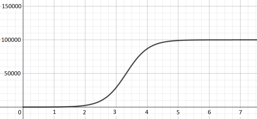
Graph H; \(\quad y(x) = \dfrac{1000000}{10 + (100000 - 10)2^{-4x}}\) The number initially increases exponentially, as the bacteria divide repeatedly, but as the number of bacteria increases the lack of food becomes an issue and so growth is much less fast.
When \(x\) is very small, the term \((10000 - 10)2^{-4x}\) is more important than \(10\) in the denominator, and \(y(x)\) is rather small (but positive).
When \(x\) is very large, the term \((10000 - 10)2^{-4x}\) in the denominator is extremely small, and so \(y(x)\) tends to \(\frac{1000000}{10}\).
Concentration in the blood of a drug following an injection.
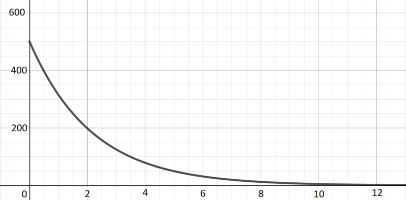
Graph G; \(\quad y(x) = 500 \times 2^{-0.6667x}\) There is a high level of the drug at the start, but it then drops off exponentially as the body metabolises the drug.
This equation corresponds to exponential decay.
Angle of oscillation of a real pendulum of length \(1\) metre in air.
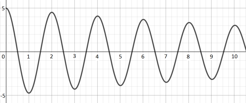
Graph C; \(\quad y(x) = 5\cos(3.13x) e^{-0.05x}\) The angle oscillates between two extremes, but those extremes become less extreme over time: the pendulum loses energy (through friction, for example) and so swings less far.
The cosine term here gives the periodic oscillation. The \(e^{-0.05x}\) gives the damping that comes from the pendulum’s loss of energy.
Volume (in litres) against pressure (in atmospheres) for \(1\) mole of an ideal gas at \(0^{\circ}\text{C}\).
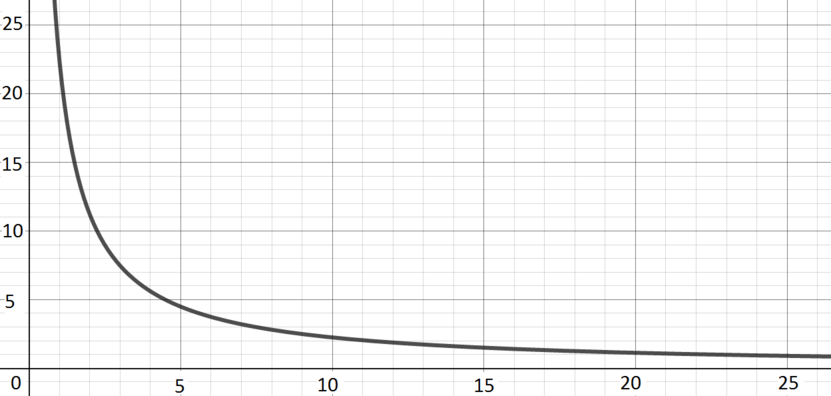
Graph I; \(\quad y(x) = \dfrac{22.4133}{x}\) Volume is inversely proportional to pressure (this makes intuitive sense, a given amount of gas takes up less volume as the pressure on it increases), so we get a reciprocal curve.)
The ideal gas law tells us that \(pV = nRT\). On the left, \(p\) is the pressure and \(V\) the volume. On the right, \(n\) is the amount of gas, \(R\) is the ideal gas constant, and \(T\) is the temperature; in our context these are all constants.
Vertical distance travelled by a small, heavy ball dropped from a plane.
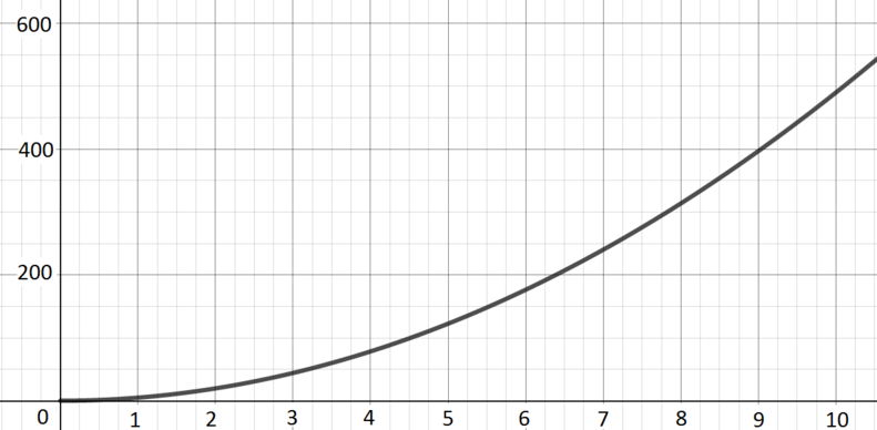
Graph B; \(\quad y(x) = 4.9x^2\) If we ignore effects of air resistance and so on, the key thing is gravity, which leads to the ball experiencing constant acceleration. This gives rise to a quadratic curve.
When the ball is dropped, we can think of it has having zero initial velocity, and its acceleration is approximately \(9.8\) metres per second per second (due to gravity), which leads to the equation (coming from \(\frac{1}{2}a x^2\)).
Rate of reaction of a catalysed reaction in terms of the concentration of reagent.
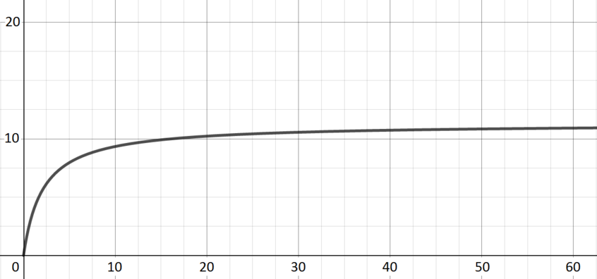
Graph E; \(\quad y(x) = \dfrac{11.3x}{2.1 + x}\) Introducing some reagent leads to a rapid increase in the rate of reaction; continuing to introduce reagent has a less dramatic effect but does still increase the rate of reaction until saturation is reached.
When \(x\) is small, the dominant term in the denominator is \(2.1\), and the function grows approximately linearly with a gradient of approximately \(5.5\).
As \(x\) increases, it becomes the more significant term in the denominator, and the function gets closer and closer to the value \(11.3\).
Number of rapidly dividing bacteria present in a food-rich environment, starting from a small initial sample.
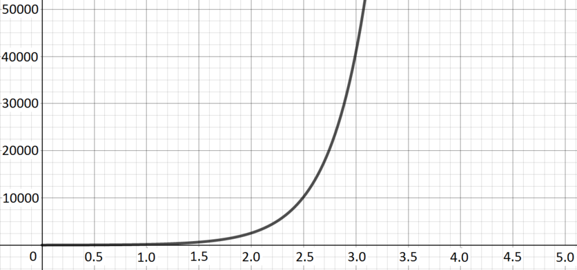
Graph D; \(\quad y(x) = 10 \times 2^{4x}\) The number of bacteria increases exponentially.
Hours of daylight per day in a town in the far northern hemisphere.
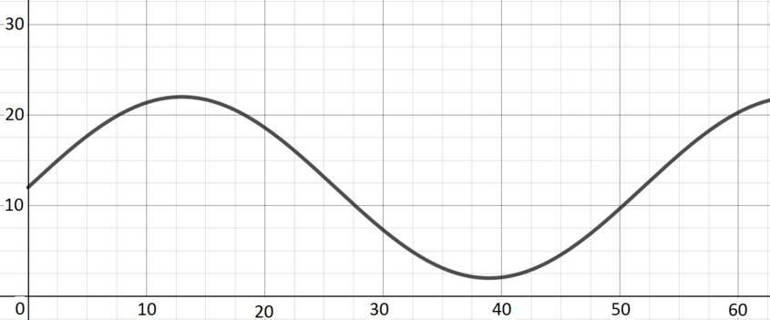
Graph F; \(\quad y(x) = 12 + 10\sin(0.121x)\) Over the course of a year, the number of hours of daylight will increase to a maximum in the middle of summer (just below \(24\)) and decrease to a minimum in the middle of winter (just above \(0\)) and return to its starting point.
The units on the horizontal axis here are weeks. This choice leads to the appearance of \(0.121\) in the argument of the sine, in order to get the right period. The number of hours of daylight varies around an average of \(12\), which is why we have a \(12\) at the beginning here, and the \(10\) scales the sine so that we get a function varying between \(-10\) and \(10\) rather than \(-1\) and \(1\).
Model of the distance of the Earth from the Sun in astronomical units.
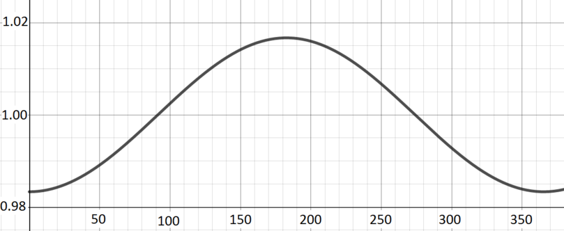
Graph A; \(\quad y(x) = 1 - 0.01671\cos(0.0172x)\) One astronomical unit is defined to be the average distance of the Earth from the Sun. As the Earth moves round the Sun in its elliptical orbit over the course of the year, it will move from slightly larger than \(1\) to slightly less than \(1\) and back again.
The units on the horizontal axis here are days, and that contributes to the \(0.0172\) in the argument of the cosine. The very small \(0.01671\) in front of the cosine reflects the fact that the Earth’s orbit is pretty close to being circular: our distance from the Sun does not change very much over the course of a year.